javaKUKA » Archive » Kinematics

This post explains position and orientation of the manipulator linkages in static situations. Kinematics, or the translations between joint angles (A1-A6) and tool positions (XYZABC), is KUKA’s backbone. This entry is of more theoretical than practical interest, as KUKA already facilitated us directly planning the tool’s motion rather than being concerned with the joint angels.

1. Transformation algebra
Translating a point leads to vector addition:

$\begin{bmatrix} x'\\ y'\\ z' \end{bmatrix} = \begin{bmatrix} \Delta x\\ \Delta y\\ \Delta z \end{bmatrix}+ \begin{bmatrix} x\\ y\\ z \end{bmatrix}$

Rotating the point about the z-axis of the coordinate system (or frame) corresponds with multiplying a rotation matrix (here we replace cos with c and sin with s):

$\begin{bmatrix} x'\\ y'\\ z' \end{bmatrix} = \begin{bmatrix} c\theta_z & -s\theta_z & 0\\ s\theta_z & c\theta_z & 0\\ 0 & 0 &1 \end{bmatrix} \begin{bmatrix} x\\ y\\ z \end{bmatrix}$

It’s convenient to put translation and rotation (about the z-axis) into one matrix:

Translation and rotation about the y-axis amounts to

$\begin{bmatrix} x'\\ y'\\ z' \\ 1 \\ \end{bmatrix} = \begin{bmatrix} c\theta_y & 0 & s\theta_y & \Delta x\\ 0 & 1 & 0 & \Delta y\\ -s\theta_y & 0 &c\theta_y & \Delta z\\ 0 & 0 &0 & 1 \end{bmatrix} \begin{bmatrix} x\\ y\\ z\\ 1 \\ \end{bmatrix} \;\;\;\; (2)$

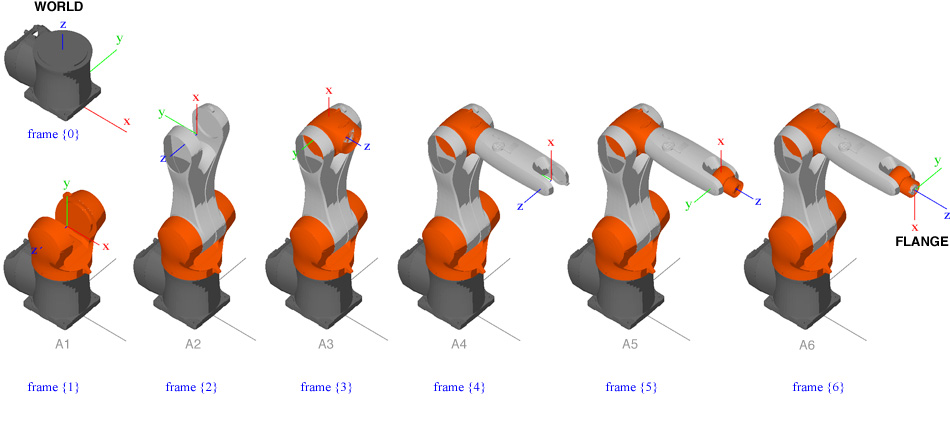
Suppose the default frame is {0}, performing transformation (1) relative to {0} leads to a new frame {1}. Performing transformation (2) relative to {1} leads to a third frame {2}. A point (x,y,z) (coordinates in {2}) has its coordinates (x’, y’, z’) in the original {0}:

$\begin{bmatrix} x'\\ y'\\ z' \\ 1 \\ \end{bmatrix} = \begin{bmatrix} c\theta_z & -s\theta_z & 0 & \Delta x\\ s\theta_z & c\theta_z & 0 & \Delta y\\ 0 & 0 &1 & \Delta z\\ 0 & 0 &0 & 1 \end{bmatrix} \begin{bmatrix} c\theta_y & 0 & s\theta_y & \Delta x\\ 0 & 1 & 0 & \Delta y\\ -s\theta_y & 0 &c\theta_y & \Delta z\\ 0 & 0 &0 & 1 \end{bmatrix} \begin{bmatrix} x\\ y\\ z\\ 1 \\ \end{bmatrix}$

We denote the matrix description of {2} relative to {0} with $^{0}_{2}T$ :

$^{0}_{2}T = \begin{bmatrix} c\theta_z & -s\theta_z & 0 & \Delta x\\ s\theta_z & c\theta_z & 0 & \Delta y\\ 0 & 0 &1 & \Delta z\\ 0 & 0 &0 & 1 \end{bmatrix} \begin{bmatrix} c\theta_y & 0 & s\theta_y & \Delta x\\ 0 & 1 & 0 & \Delta y\\ -s\theta_y & 0 &c\theta_y & \Delta z\\ 0 & 0 &0 & 1 \end{bmatrix}$

The principle is that the matrix of a successive transformation is at the right side of the multiplication:

$^{0}_{2}T = {^{0}_{1}T} \;{^{1}_{2}T} \;\;\;\; (3)$

2. Forward kinematics
Following the rule of compound transformation (3), it is straightforward to computer $^{0}_{6}T$ , namely, the description of the FLANGE {6} relative to the WORLD {0}:

$^{0}_{6}T ={^{0}_{1}T}\;{^{1}_{2}T}\;{^{2}_{3}T}\;{^{3}_{4}T}\;{^{4}_{5}T}\;{^{5}_{6}T}$

Where the six matrices are given by ( $c_i$ stands for $\cos(\theta_i)$ and $s_i$ stands for $\sin(\theta_i)$ )

$^{0}_{1}T =\begin{bmatrix} c_0 & 0 & s_0 & a_0 c_0\\ s_0 & 0 &-c_0 & a_0 s_0\\ 0 & 1 &0 & d_0 \\ 0 & 0 &0 & 1 \end{bmatrix} \;\;\;\;\; ^{1}_{2}T =\begin{bmatrix} c_1 &-s_1 & 0 & a_1 c_1\\ s_1 &c_1 & 0 & a_1 s_1\\ 0 & 0 &1 & d_1 \\ 0 & 0 &0 & 1 \end{bmatrix} \;\;\;\;\; ^{2}_{3}T =\begin{bmatrix} c_2 & 0 & s_2 & a_2 c_2\\ s_2 & 0 &-c_2 & a_2 s_2\\ 0 & 1 &0 & d_2 \\ 0 & 0 &0 & 1 \end{bmatrix}$

$^{3}_{4}T =\begin{bmatrix} c_3 & 0 &-s_3 & a_3 c_3\\ s_3 & 0 &c_3 & a_3 s_3\\ 0 & -1 &0 & d_3 \\ 0 & 0 &0 & 1 \end{bmatrix} \;\;\;\;\; ^{4}_{5}T =\begin{bmatrix} c_4 & 0 & s_4 & a_4 c_4\\ s_4 & 0 &-c_4 & a_4 s_4\\ 0 & 1 &0 & d_4 \\ 0 & 0 &0 & 1 \end{bmatrix} \;\;\;\;\; ^{5}_{6}T =\begin{bmatrix} c_5 &-s_5 & 0 & a_5 c_5\\ s_5 &c_5 & 0 & a_5 s_5\\ 0 & 0 &1 & d_5 \\ 0 & 0 &0 & 1 \end{bmatrix}$

Where $a_i$ and $d_i$ (i=0,1,.., 5) are the DH (Denavit–Hartenberg) parameters that describe the dimensions of the each linkage of the robot.

For instance, the DH parameters of KR6 R900 are:
a = { 25, 455, 35, 0, 0, 0 };
d = { 400, 0, 0, 420, 0, 80 };

Likewise, the DH parameters of KR16 are:
a = { 260, 680, -35, 0, 0, 0 };
d = { 675, 0, 0, 670, 0, 158 };

ABB IRB 4600-45/2.05:
a = { 175, 900, 175, 0, 0, 0 };
d = { 495, 0, 0, 960, 0, 135 };

These data agree with the robot’s dimensions, which can be found in the data sheet.

Now, we use forward kinematics to visualize robot’s body in Java. The pedestal is directly rendered in frame {0} (WORLD), which is the default coordinate system of Java’s virtual 3D scene. As the first link resides in frame {1}, we need to transform the geometry of the link before drawing it in the frame {0}:

$\begin{bmatrix} x'\\ y'\\ z' \\ 1 \\ \end{bmatrix} = {^{0}_{1}T} \begin{bmatrix} x\\ y\\ z\\ 1 \\ \end{bmatrix}$

where x, y, z are the coordinates of the vertices of the link’s geometry, relative to itself (the link’s bottom center is located at (0,0,0)); while x’, y’, z’ are the coordinates of the link in the frame {0}, so we can render all the vertices (x’, y’, z’) in {0} correctly.

The vertices of the second link are given by

$\begin{bmatrix} x'\\ y'\\ z' \\ 1 \\ \end{bmatrix} = {^{0}_{1}T}\;{^{1}_{2}T} \begin{bmatrix} x\\ y\\ z\\ 1 \\ \end{bmatrix}$

Likewise for other succeeding links. Finally, the position of the flange (the sixth link) would be

$\begin{bmatrix} x'\\ y'\\ z' \\ 1 \\ \end{bmatrix} = {^{0}_{6}T} \begin{bmatrix} x\\ y\\ z\\ 1 \\ \end{bmatrix}$

As such, one can visualize the links one by one using the transformation matrices $^{0}_{i}T$ for i=1, 2,…6:

DisplayKuka (dependencies: Processing and Peasycam) demonstrates the forward kinematics using a 3D model of KR6 R900. Please download the 3D model (and unzip) and place it in the bin folder (Eclipse).

Our Robot class provides the function double[][] forward(double[] ts) whose input is the joint angles in radius, and output is the matrix $^{0}_{6}T$ .

Another function double[][][] forwardSequence(double[] ts) returns the six matrices: $^{0}_{1}T$ , $^{0}_{2}T$ , $^{0}_{3}T$ , $^{0}_{4}T$ , $^{0}_{5}T$ , and $^{0}_{6}T$ .

3. BASE & TOOL
XYZABC and transformation matrix are two exchangeable representations of transformations (methods for conversion can be found in the LA class). When navigating to Start-up / Calibrate / BASE (or TOOL) / Numeric input, we can see the BASE or the TOOL represented by XYZABC, which is equivalent to the matrix representation.

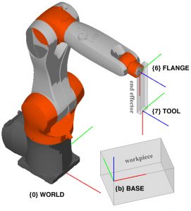
$^{0}_{b}T$ denotes the BASE frame relative to WORLD. Regarding the tool as the 7th link, we denote the TOOL frame (relative to FLANGE) as $^{6}_{7}T$ , as a result:

${^{0}_{b}T}\;\;{^{b}_{7}T} = {^{0}_{6}T} \;\; {^{6}_{7}T}$

${^{b}_{7}T} = \left( ^{0}_{b}T \right)^{-1} {^{0}_{6}T} \;\; {^{6}_{7}T}$

where $^{b}_{7}T$ is the very data that one mostly cares for, because $^{b}_{7}T$ tells how the tool is located in the BASE (usually corresponds to the workpiece). Notice that a typical KRL command PTP {X 280, Y 0, Z -10, A 30, B 90, C 0} specifies the tool’s position in the BASE.

The Robot class provides a method double[] forward(double[] degs, double[][] base, double[][] tool) which converts joint angles A1-A6 (with TOOL and BASE) to $^{b}_{7}T$ (in the form of XYZABC).

Here is a simple example testing forward kinematics :
double[] a = { 260, 680, -35, 0, 0, 0 };
double[] d = { 675, 0, 0, 670, 0, 158 };
Robot kr=new Robot(a,d); //KR 16
double[] degs = {35.55, -54.91, 88.58, 62.39, 39.19, -32.95 }; //A1-A6
double[][] tool = LA.matrix(-54.707, -59.723, 77.7, -11, 22, -33);
double[][] base = LA.matrix(898.094, -1265.699,245.752,161.956,-11,22);
double[] results = kr.forward(Robot.DegToRad(degs, “KUKA”), base, tool);

4. Inverse Kinematics
Opposite to forward kinematics, inverse kinematics calculates joint angels (A1-A6) from tool positions (XYZABC). Given a flange position XYZABC (corresponds to $^{0}_{6}T$ ), there could be multiple solutions of joint angles. KUKA uses S and T parameters to reduce ambiguity. The following image shows four configurations of joint angles with the same position $p_5$ .

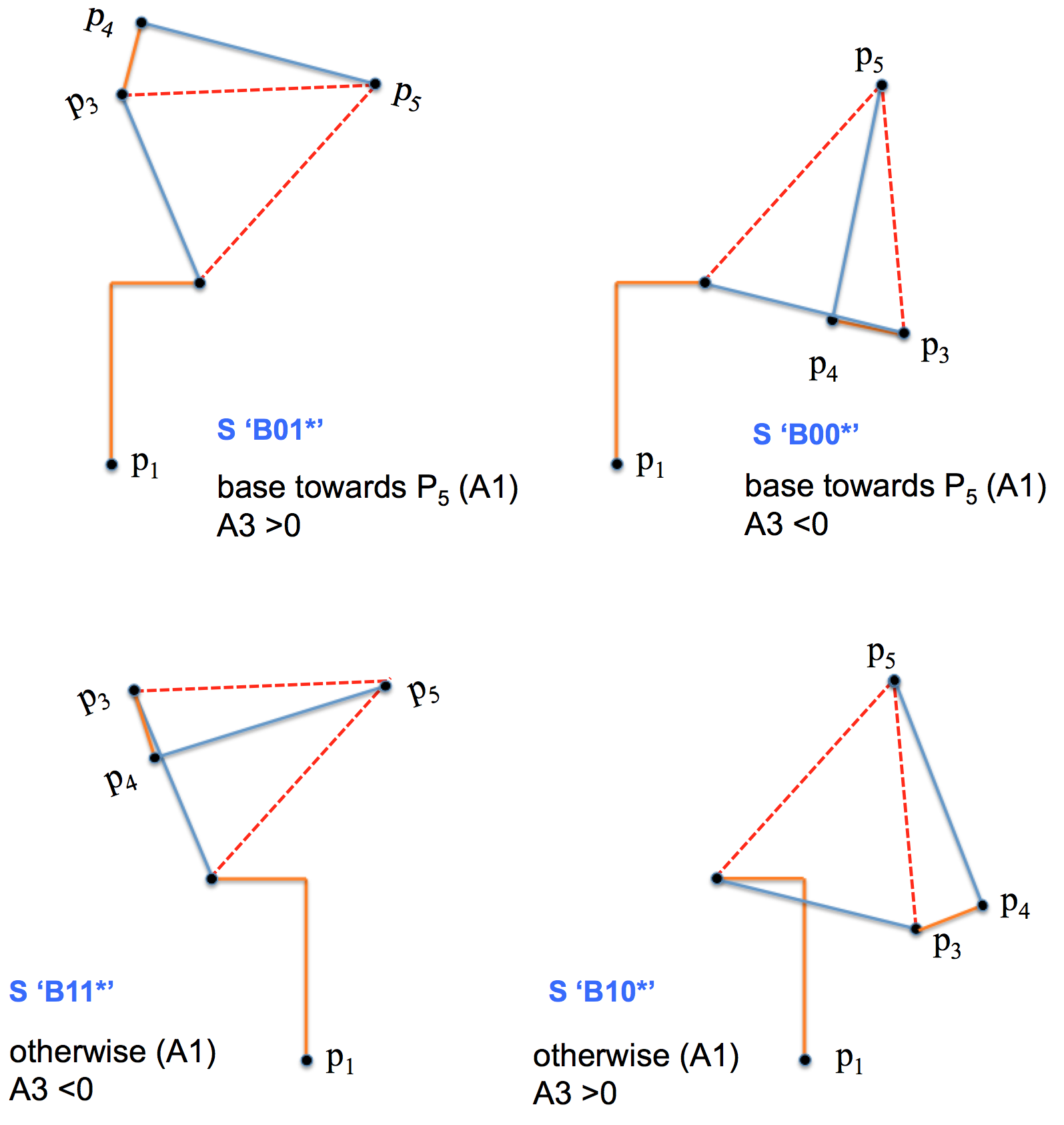
The robot arm has a characteristic feature: the center of the fifth joint ( $p_5$ ), as well as $p_1$ , $p_2$ , $p_3$ , and $p_4$ , always lies on the XZ plane of the first joint. Therefore angle A1 is obtained by

$\theta_0 (A1)= \tan^{-1}(p_{5y},p_{5x})$

$p_5={^{0}_{6}T} \begin{bmatrix} 0\\ 0\\ -d_5 \\ 1 \end{bmatrix}$

Within the XZ plane, one can employ geometric method to find A2 and A3 (multiple values possible). The following image shows the robot skeleton in the XZ plane (orthogonal to the XY plane of WORLD) of the first joint.

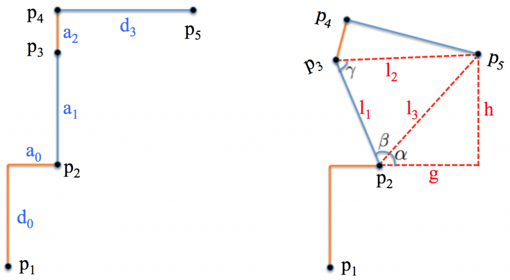
First we compute $\alpha$ :

$\alpha= \tan^{-1}(h,g)$

$h=p_{5z}-d_0$

$g=s||p_{5xy}-p_{2xy}|| \;\;\;\; s= \begin {cases} 1 \;\; if \;(p_{5xy}-p_{2xy})\cdot(p_{1xy}-p_{2xy})<0\\ -1 \;\;otherwise\\ \end{cases}$

where $(\cdot)_{xy}$ denote the projection of a vector onto the XY plane of WORLD. Notice that $p_2$ is available once A1 is obtained. Then we compute

$\beta=\cos^{-1} \left( \frac{l_1^2+l_3^2-l_2^2}{2l_1 l_3} \right)$

$\gamma=\cos^{-1} \left( \frac{l_1^2+l_2^2-l_3^2}{2l_1 l_2} \right)$

so A2 and A3 are given by

$\theta_1 (A2)= \alpha+\beta$

$\theta_2 (A3)= \gamma- \tan^{-1}(a_2,d_3)- \frac{\pi}{2}$

Notice that the above formula only gives one possible pair of A2-A3 values that lead to a given position $p_5$ .

Now, we take an algebraic approach to find A4, A5, and A6. First, one can obtain the matrix’s value:

${^{3}_{6}T}= ({^{0}_{3}T})^{-1} \;\; {^{0}_{6}T}$

since $^{0}_{3}T$ could be computed from A1, A2, and A3. Based on the following equation:

${^{3}_{6}T} =\begin{bmatrix} c_3 & 0 &-s_3 & a_3 c_3\\ s_3 & 0 &c_3 & a_3 c_3\\ 0 & -1 &0 & d_3 \\ 0 & 0 &0 & 1 \end{bmatrix} \begin{bmatrix} c_4 & 0 & s_4 & a_4 c_4\\ s_4 & 0 &-c_4 & a_4 s_4\\ 0 & 1 &0 & d_4 \\ 0 & 0 &0 & 1 \end{bmatrix} \begin{bmatrix} c_5 &-s_5 & 0 & a_5 c_5\\ s_5 &c_5 & 0 & a_5 s_5\\ 0 & 0 &1 & d_5 \\ 0 & 0 &0 & 1 \end{bmatrix} \;\;\;\;(4)$

we finally arrive at the angels A4-A6:

$\theta_3 (A4)=\tan^{-1}(^{3}_{6}T_{12},\; ^{3}_{6}T_{02})$

$\theta_4 (A5)=\cos^{-1} ({^{3}_{6}T_{22} })$

$\theta_5 (A6)=\tan^{-1}(^{3}_{6}T_{21},\; -^{3}_{6}T_{20})$

Equation (4) indicates that $^{3}_{6}T$ is a function of A4, A5, and A6. It is easy to find the following invariance:

$^{3}_{6}T(A4, A5, A6) =\; ^{3}_{6}T(A4 \pm 180, -A5, A6 \pm 180)$

which leads to multiple solutions of A4, A5, and A6 given a specific $^{3}_{6}T$ .

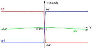
Additional care should be taken for singularity ( $^{3}_{6}T_{22}=1$ ). The following graph shows that the mapping from a Cartesian position (of flange) to joint angles is not necessarily smooth. The origin of graph is the HOME position (flange’s position in WORLD). When the flange move slightly toward the positive (or negative) y-axis of WORLD, A4 and A5 change extremely quickly to $\pm \pi/2$ .

The following Java codes (or download TestInverse) illustrate how to perform inverse kinematics with the Robot class:
double[] a = { 25, 455, 35, 0, 0, 0 };
double[] d = { 400, 0, 0, 420, 0, 80 };
Robot kr = new Robot(a, d); // KR6 R900

double[] position = { 525, 0, 890, 0, 90, 0 }; // xyzabc, HOME position, flange’s position in WORLD
double[] theta = kr.inverse(position, new Double(0), null, null);
double[] angles = Robot.RadToDeg(theta, “KUKA”);

References:
J. J. Graig, Introduction to Robotics, chapters 2,3,4.
P. Schneider and D. Eberly, Geometric Tools for Computer Graphics, chapters 2,3,4.

javaKUKA play KUKA in Java

Kinematics