javaKUKA » Archive » Minimal Surfaces

This post shows an algebraic approach to robotic fabrication. The desirable tangent vector of the tool, expressed in a closed-form, directly specifies the robot codes (KRL) for hot-wire cut. This is a radical demonstration of how javaKUKA manages toolpath planning without 3D representation of the workpiece or using industrial CAM software. The product (workpiece) is the exact consequence of physical toolpath; the 3D model (e.g., mesh) is a biased representation of virtual toolpath. So we regard the tool trajectory instead of the workpiece geometry as the first-class citizen in design & fabrication.

1. Minimal surfaces
The Weierstrass representation is a generic model for all minimal surfaces. It defines a minimal surface $X$ ( $\mathbb{R}^3$ ) on a complex plane ( $\mathbb{C}$ ). Let $\omega=u+v i$ (the complex plane as the $uv$ space), we write the Jacobian matrix of the surface as a column of complex entries:

$\mathbf{J}= \begin{bmatrix} \left( 1- g^2(\omega) \right)f(\omega) \\ i\left( 1+ g^2(\omega) \right)f(\omega) \\ 2g(\omega) f(\omega) \end{bmatrix} \quad (1)$

The Jacobian $\mathbf{J}$ represents the two orthogonal tangent vectors of the surface:

$\mathbf{X_u}= \begin{bmatrix} \operatorname{Re}\mathbf{J}_1 \\ \operatorname{Re}\mathbf{J}_2 \\ \operatorname{Re} \mathbf{J}_3 \end{bmatrix} \;\;\;\; \mathbf{X_v}= \begin{bmatrix} -\operatorname{Im}\mathbf{J}_1 \\ -\operatorname{Im}\mathbf{J}_2 \\ -\operatorname{Im} \mathbf{J}_3 \end{bmatrix}$

The surface normal is

$\mathbf{\hat{n}}= \mathbf{X_u}\times \mathbf{X_v}= \frac{1}{| g|^2+1} \begin{bmatrix} 2\operatorname{Re} g\\ 2\operatorname{Im} g \\ | g|^2-1 \end{bmatrix} \quad (2)$

A point $\omega_t$ on the complex plane maps to a point $\mathbf{X}$ on the minimal surface in $\mathbb{R}^3$ by

$\mathbf{X}= \begin{bmatrix} \operatorname{Re} \int_{\omega_0}^{\omega_ t}\mathbf{J}_1 d\omega\\ \operatorname{Re} \int_{\omega_0}^{\omega_ t} \mathbf{J}_2 d\omega\\ \operatorname{Re} \int_{\omega_0}^{\omega_ t} \mathbf{J}_3 d\omega \end{bmatrix} \quad (3)$

The Weierstrass model yields immersed minimal surfaces; however, it does not address the problem of self-intersections. An important method is using the fundamental patch to construct periodic minimal surfaces. The infinite continuous surface is constructed from copies of the fundamental patch by translation, rotation and reflection. Classical examples include Schwarz surfaces and Scherk’s surfaces.

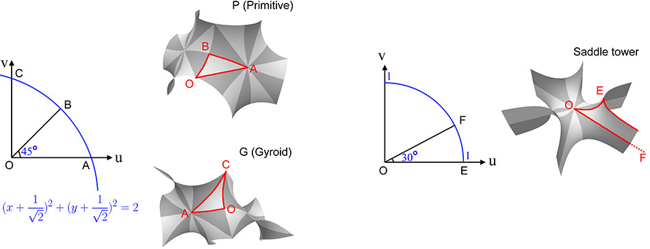
Fig.1 The affine transformed copies of the fundamental patch span the continuous Triply Periodic Minimal Surfaces (TPMS).

2. Parameterization with principal directions
One has to subdivide the infinitely extensible PMS into manageable workpieces for wire-cut machines. Now we focus on the workpiece reparameterization from which the toolpath can be directly derived. Although the surface is smooth across the boundary of fundamental patches, the $uv$ lines are not $C^1$ smooth across the fundamental patches, which is unacceptable for wire cut (a workpiece usually consists of multiple fundamental patches). Our reparameterization defines a smooth cross field (orthonormal frame field) on the surface. The pair of orthogonal tangents at each position corresponds to the cutting wire’s orientation and its velocity vector (normalized) respectively. The principal directions and the normal span a local orthonormal basis. The lines of curvature are smooth everywhere on the surface except for singular points.

One can relate the new orthogonal coordinates $(\sigma,\tau)$ to the original $(u,v)$ coordinates by a direction field $\phi(u,v)$

$\tan^{-1}\left(\frac{\partial\sigma}{\partial v},\frac{\partial\sigma}{\partial u} \right)=\phi(u,v) \quad (4)$

Because the map (1) from the $uv$ domain to the 3D surface is conformal, the tangent vectors with respect to the $(\sigma,\tau)$ parametrization are given by

$\mathbf{X_\sigma}= \cos\phi \mathbf{X_u}+ \sin\phi \mathbf{X_v},\quad \mathbf{X_\tau}= -\sin\phi \mathbf{X_u}+ \cos\phi \mathbf{X_v} \quad (5)$

$\mathbf{X_\sigma}$ and $\mathbf{X_\tau}$ happen to be the principal directions if $\phi$ complies with equation (5).

One principal direction in the complex domain is

$\overline{\sqrt{ f g'} }\quad (6)$

Therefore, the two principal directions in the $uv$ space turn out to be

$\phi= -\frac{1}{2} Arg(f g') \pm k \pi /2$

The cross field identifies the ( $\sigma,\tau$ ) coordinates according to (4). Consequently, one can compute the principal directions $\mathbf{X_\sigma}$ and $\mathbf{X_\tau}$ by (5). One can use Runge-Kutta method to construct two sets of orthogonal streamlines in the 2D field $\phi$ , and the corresponding 3D streamlines (on the surface) as the trajectories of wire cutting (Fig.2).

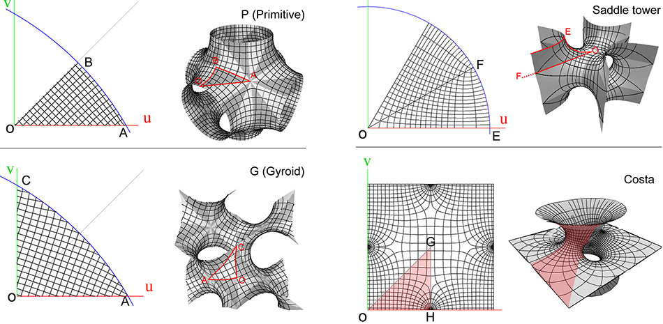
Fig.2 Lines of curvature (6) make a quadrangulation of the domain.

(6) gives an algebraic expression for the principal direction of any minimal surface, once the holomorphic functions $f(\omega)$ and $g(\omega)$ are given. For instance, the principal direction of Schwarz P surface is

$\overline{(\omega^8-14\omega^4+1)^{-1/4}}$

Likewise, Saddle tower’s (Scherk surface $k=3$ ) principal direction is

$\overline{\omega^{1/2}(\omega^6+1)^{-1/2} }$

The principal direction of Costa’s surface is given by

$\overline{-\wp (\wp')^-2 \wp''}= \overline{(3\wp^2- e_1^2)/(e_1^2-\wp^2)}$

where $e_1$ is constant and $\wp(\omega)$ denotes Weierstrass’s elliptic function.

The complex domains of the surfaces can be quadrangulated according to the principal directions (Fig.2).

3. Double-sided cutting scheme
A family of ruled surfaces can offer an approximation of a minimal surface. A sufficiently long wire cannot cut double-sided surfaces of positive Gaussian curvature without collisions. For instance, wire cutting can approximate the outside surface of a piece of an egg shell; however, it would be impossible to produce the inside surface.

A global quadrangulation ( $\sigma\tau$ -lines) enables us to complete the wire cutting of a workpiece in three steps (Fig.3):
1) front cut: aligning the wire with $\mathbf{X_\sigma}$ when the wire travels along $\mathbf{X_\tau}$ -lines.
2) back cut: aligning the wire with $\mathbf{X_\tau}$ when the wire travels along $\mathbf{X_\sigma}$ -lines.
3) side cut: aligning the wire with $\hat{\mathbf{n}}$ when the wire cuts the boundary.

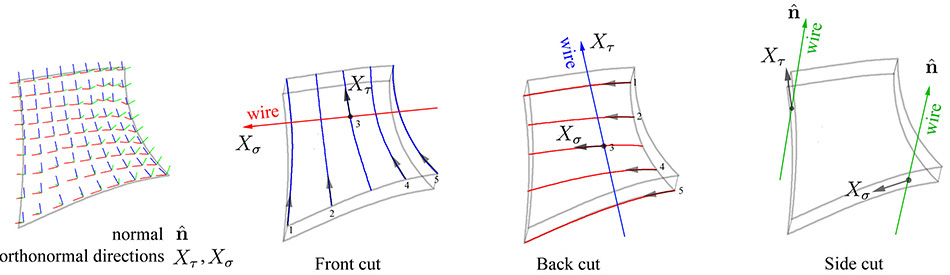
Fig.3 The orthogonal double-sided cuts correspond to the orthonormal directions $\mathbf{X_\sigma}$ , $\mathbf{X_\tau}$ , and $\hat{\mathbf{n}}$ on the surface.

Orthogonality: on any point on the surface, the line cutting one side of the surface is orthogonal to that on the other side. Further, the velocity vector (or, the cutting direction) of the line cutting one side of the surface is orthogonal with that on the other side.
Interchangeability: swapping the wire’s velocity vector with its orientation (in other words, swapping the values of $\mathbf{X_\sigma}$ and $\mathbf{X_\tau}$ ) leads to a mirrored copy of the original workpiece.

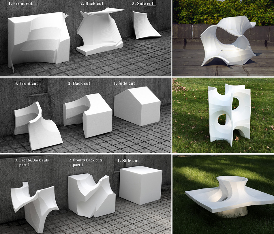
Fig.4 Top row: cutting a workpiece (equivalent to two fundamental patches) of Gyroid surface (left), and the assembly of 20 workpieces (right). Middle row: cutting a workpiece (equivalent to four fundamental patches) of the Saddle tower (left), and the assembly of 9 workpieces (right). Bottom row: cutting a workpiece (equivalent to two fundamental patches) of Costa’s minimal surface (left), and the assembly of 4 workpieces (right).

4. Hot-wire cutting
Mounting a hotwire tool to a robot arm leads to a flexible cutter. Both position (XYZ) and orientation (ABC: Euler angles) identify the geometric state of the tool (hotwire). Suppose the center of the tool is predefined on the wire (e.g. at the wire’s midpoint), the cutting position for a given point on the streamlines is given by

$\begin{bmatrix} X \\ Y \\ Z \end{bmatrix} =M(\mathbf{ X})s+ m(\hat{ \mathbf{n}})h \quad (7)$

Where $s$ denotes the global scalar for the workpiece, $h$ denotes workpiece’s (half) thickness; $m( )$ denotes reflection and rotation for $\mathbf{X_\sigma},\mathbf{X_\tau}$ and $\hat{ \mathbf{n}}$ ; $M( )$ denotes reflection, rotation and translation for the point $\mathbf{X}$ on the surface.

To specify the wire’s orientation, we first put the local orthonormal vectors $\mathbf{X_\sigma},\mathbf{X_\tau}$ and $\hat{ \mathbf{n}}$ into a unitary matrix

$\mathbf{T}= \begin{bmatrix} \mathbf{X_\sigma}_x & \mathbf{X_\tau}_x &\hat{ \mathbf{n}}_x \\ \mathbf{X_\sigma}_y & \mathbf{X_\tau}_y &\hat{ \mathbf{n}}_y \\ \mathbf{X_\sigma}_z & \mathbf{X_\tau}_z &\hat{ \mathbf{n}}_z \\ \end{bmatrix}$

then Z-Y-X Euler angles (ABC) can be found by solving the following equation

$\begin{bmatrix} cA &-sA &0 \\ sA &cA &0 \\ 0 & 0 & 1 \end{bmatrix} \begin{bmatrix} cB & 0 & sB \\ 0 & 1 & 0 \\ -sB & 0 &cB \end{bmatrix} \begin{bmatrix} 1 & 0 & 0 \\ 0 & cC &-sC \\ 0 & sC &cC \end{bmatrix} =\mathbf{T} \quad (8)$

where $c$ and $s$ denote $\cos$ and $\sin$ respectively.

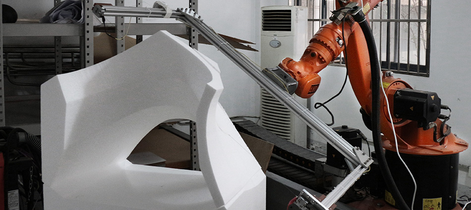
Fig.5 Cutting a “saddle tower” workpiece with the robotic system in our workshop. A hotwire tool is mounted to the flange of the KUKA robot.

A KUKA robot can approximate a continuous cut (following a $\mathbf{X_\sigma}$ or $\mathbf{X_\tau}$ line) by a set of linear movements (LIN) or by a spline movement (SPLINE). We implemented KUKA’s spline movement whose key points are specified in the form of

SPL { X_ Y_ Z_ A_ B_ C_ }

As a result, the XYZABC values for SPL commands are directly obtained from the closed-form expression of the toolpath (7)(8).

Summary
This application shows a possibly shortest path from a mathematical formulation of workpiece geometry to the data in the robot instructions that result in the geometry. The design & toolpath planning mainly consist of:
(1) Designing and describing the workpiece via a structured family of toolpaths, each of which is defined by a mathematical expression.
(2) Sampling the data points from the mathematical expressions, and feeding them into the robot commands.

Thus we are looking for the geometric & topological fit between the predefined types of robot motions and the workpiece design.

References:
[1] Nitsche, J.C., 1989. Lectures on minimal surfaces: vol. 1. Cambridge university press.
[2] Gandy, P.J. and Klinowski, J., 2000. Exact computation of the triply periodic G (Gyroid’) minimal surface. Chemical Physics Letters, 321(5-6), pp.363-371.
[3] Meeks III, W. and Pérez, J., 2011. The classical theory of minimal surfaces. Bulletin of the American Mathematical Society, 48(3), pp.325-407.
[4] Osserman, R., 2013. A survey of minimal surfaces. Courier Corporation.
[5] Hua, H. and Jia, T., 2018. Wire cut of double-sided minimal surfaces. The Visual Computer, 34(6-8), pp.985-995

javaKUKA play KUKA in Java

Minimal Surfaces